The strangeness of Entanglement

for beginners...

In the last century physicists have developed quantum mechanics, a theory required to explain observations made at the atomic level. Quantum mechanics is a very successful theory: It can precisely predict the colours emitted by atoms and give an explanation for the properties of the elements. It also describes a property discovered in quantum system called "entanglement", but in doing so it forces us to reject locality or reality.

Our common experience of the world is local and real. It is taught to us by experience and expressed with statements such as: "Touch the cup of tea to feel if it's warm" or "The gold is in the safe."

Locality expresses a known interaction observed between two objects when they touch each other. This interaction allows two objects to influence each other in a predictable way. Your hand must touch the cup of tea to feel the warmth.

Reality expresses a relationship between our knowledge and the world. When something is real our knowledge of it can be demonstrated. Open the safe and you will find the gold.

Entanglement is a statistical property of quantum systems. Because entanglement is not observed in familiar objects, it is a concept which might be difficult to grasp. Its description involves statistical analysis, quantum mechanics and Bell's inequalities. In this paper, however, I present entanglement from a simpler point of view. The statistical analysis is simplified to a level comparable in difficulty with the analysis of a coin toss or a roll of the die. Moreover, most of the difficulties related to quantum mechanics are avoided by using a much more familiar classical scenario.

The scenario of a classical experiment is presented first. Based on locality and reality, only one model explains the experimental results. Then, the model is used to make a complementary prediction which is confirmed by the results. In the second part of this paper, a quantum experiment is described where entanglement is observed. The description is phenomenological and does not require a knowledge of quantum mechanics beyond what is expected from the reader. However, since this quantum experiment was carried out in a laboratory, results are available for this discussion. Based on locality and reality, the experimental results are explained by only one model which turns out to be the same model found for the classical scenario.

Because of the strange properties of entanglement, however, the complementary predictions made by the model disagree with the results of the quantum experiment. The only explanation for the discrepancy is that locality or reality must be rejected.

This is inspired by the papers from Mermin[1] and Bell[2].

A classical experiment

1) Classical experiment and correlations

Imagine this scenario which describes a classical experiment: Three people are involved in this experiment: you, myself and a common friend who writes to both of us. Each week our friend sends a pair of postcards, one for you and the other one for me. Both postcards are sent at the same time via Canada Post. In this scenario, the mail service is the fastest way to communicate between people: it takes at least two days to deliver the mail, but never more than three.

Upon receiving several postcards, I observe the following. The postcards always have three flaps labeled 1, 2 and 3 and a date written on the postmark. When a flap is lifted a single word is exposed which can be either "heads" or "tails". However, the postcards have a special mechanism: Opening a flap makes ink flow behind the other two and covers the other words. So although I am free to choose which flap to lift, I can only read one of the three words.

Having figured out so much, I decide to start recording my data in a systematic way. Upon receiving the postcard, I pick a random number from 1 to 3 and lift the flap labeled with that number. On the first week I choose the number 1 and lift the corresponding flap; the word "heads" appears. The next week, I choose 3 and the word "heads" appears. The following postcard has "tails" underneath flap 1. After two months my list of flap-numbers and words is: 1H, 3H, 1T, 1H, 2H, 2T, 3H, 3H.

I am intrigued by the behaviour of our friend and wonder what he writes on your postcards. So I send you my list (also via Canada post) with the date of the first entry. Since great minds think alike, you also have been recording data obtained by lifting flaps at random. You send me your data, starting on the same date as mine: 2H, 3H, 3H, 1H, 1T, 2T, 1H, 2T.

Being an investigative person, you combine our lists to make word-pairs with my data on the left and yours on the right: 1H2H, 3H3H, 1T3H, etc. You discover something interesting: Word-pairs with the same flap-numbers always have the same words! The combined observations give the following word-pair list:

1H2H 3H3H <- flap 3 lifted on both postcards, same words exposed: "heads" and "heads" 1T3H 1H1H <- flap 1 lifted on both postcards, same words exposed: "heads" and "heads" 2H1T 2T2T <- flap 2 lifted on both postcards, same words exposed: "tails" and "tails" 3H1H 3H2T
This continues for several years until we each have received over 400 such postcards. We combine our lists to get the word-pairs shown below in Table 1. Although the words "heads" and "tails" seem to be randomly distributed, word-pairs with the same flap-numbers always have the same words! They are highlighted in red to make them stand out.

TABLE 1. Partial list of 432 word-pairs from the postcards received every week. The green rectangle highlights my
first entries. The red entries are those for which we randomly chose the same flap-numbers.

This is an example of a correlation: it is a predictable relationship between two different data. The correlation is perfect for word-pairs with the same flap-number because we can predict with 100% certainty that the outcome will be a word-pair with the same words.

2) Statistical analysis

A statistical analysis is necessary to better understand random data. The analysis gives the probability of obtaining a certain outcome in a large data set. A probability is the ratio of two numbers: the number of desired outcomes and the number of all possible outcomes.
For example, the theoretical probability of winning a coin toss if you bet "heads" is calculated as follows. The number of desired outcomes is 1 since there is only one outcome that can make you win. The total number of possible outcomes is 2 since the coin has a total of two sides, "heads" or "tails". The probability of winning is 1÷2 = 50%.
Another example: what is the probability of throwing "4" or "5" with a single die? The number of desired outcomes is 2 since there is one "4" and one "5" on the die. The total number of possible outcomes is 6 since a die has six sides. The probability of throwing a "4" or a "5" is 2÷6 = 33.3%.
In an actual experiment, the number of occurrence of a desired outcome must be counted on a large number of measurements to obtain a good estimate of the probability. For example, you might toss a coin 1000 times and obtain 489 "heads". The estimated probability of getting "heads" is 489÷1000 = 48.9%, which is consistent with the 50% probability calculated from a fair coin. The estimate is less accurate if fewer measurements are available.

After eight years of receiving postcards from our (boring) friend, we make a statistical analysis of the entries in Table 1.

A) For this first analysis we only look at individual entries.
Although this analysis is overwhelming, the important thing to retain is that the estimated probabilities are all consistent with a probability of 50%.

Counting the entries in my list where I lifted flap 1: 1H is listed 78 times, 1T is listed 67 times, for a total of 145 words. Therefore the estimated probability of occurrence for "heads" is 78÷145 = 54% and for "tails" is 67÷145 = 46%.
The same procedure gives for my other entries: 2H = 50%, 2T = 50%, 3H = 43%, 3T = 57%, and independently of the flap I chose H = 49%, and T =51%. For your entries: 1H = 49%, 1T = 51%, 2H = 56%, 2T = 44%, 3H = 40%, 3T = 60%, H = 48%, and T =52%.
If all entries are taken together, the estimated probability of occurrence for "heads" is 48.6% and for "tails" is 51.4%.

B) For this second analysis we look at the combined word-pair entries, but only those with the same flap-numbers.
Word-pairs having the same words are listed 139 times, word-pairs having different words are not found in the list, for a total of 139 word-pairs with the same flap-numbers (shown in red in Table 1 as 1T1T, 1H1H, 2T2T, 2H2H, 3T3T, and 3H3H).
The estimated probability of occurrence of the same words when the same flap-numbers are chosen is 139÷139 = 100%.

3) A model for the observed statistics and correlations

We explain these results by following this formal line of reasoning.

A) The conditions of the classical experiment are:
i- A postcard has three flaps, each one hides a single word: "heads" or "tails".
ii- Lifting a flap exposes a word and releases ink that covers the other two, making them unreadable.
iii- Our friend sends pairs of postcards simultaneously via Canada Post, one for you the other for me. A postmark with the sent date is printed on the postcards.
iv- It takes at least two days to deliver the mail, never more than three. This is the fastest way to communicate between each other.
v- A random number is chosen just before lifting the flap labeled with that number. This is done in order to sample the words without any bias.
vi- For every postcard I take note of the date, the chosen flap-number and the exposed word. You follow the same procedure.
vii- There is no other common agreement between any of you, me and our friend.
viii- There is no communication between any of us except for:
   - the postcards sent to us by our friend,
   - the lists sent to each other.
ix- Our lists are combined into word-pairs for each pair of postcards sent on the same date.

B) The individual observations are:
i- One of only two possibilities, "heads" or "tails", is exposed when a flap is lifted. We never see an ink covered word.
ii- The occurrence of the words is random, with no discernible pattern.
iii- The words have a near equal chance of being used, independently of which flap is lifted. This is the result of the statistical analysis (2A).

C) The combined observations are:
i- Word-pairs with the same flap-number always have the same words. This is the result of the statistical analysis (2B).

D) We make a few (reasonable but debatable) assumptions:
i- Our friend flips a coin to generate the random words on the postcards. The statistical analysis (2A) is consistent with the 50% probability expected from a coin toss.
ii- The word exposed when I lift a flap tells me that a the same word is written in your postcard under the same-numbered flap, even if you never lift that flap.
   (What Einstein called "element of reality": the word is determined even if nobody looks. "The moon is there when nobody looks.")
iii- Since I am free to choose which flap to lift, all three words on your postcard must already be determined when the postcard is sent.
   This is because it is potentially possible for me to predict which word will be written under any of your flaps.
iv- You can deduce the same thing about the words written in my postcard.
v- Transmission of information is impossible at a speed faster than Canada Post can send a message.
   ("Locality" is assumed: a message cannot influence the other at another location faster than the maximum speed of transmission of messages.)

E) Given that we accept what is written above, we conclude the following:
i- In order to explain observation (3C-i), our friend must send us identical postcards chosen from one of these eight templates. There is no other possibility.

Template   My postcard    Your postcard 1    1H - 2H - 3H    1H - 2H - 3H 2    1H - 2H - 3T    1H - 2H - 3T 3    1H - 2T - 3H    1H - 2T - 3H 4    1H - 2T - 3T    1H - 2T - 3T 5    1T - 2H - 3H    1T - 2H - 3H 6    1T - 2H - 3T 1T - 2H - 3T 7    1T - 2T - 3H    1T - 2T - 3H 8    1T - 2T - 3T    1T - 2T - 3T

ii- Each template has the same probability of being chosen. This is necessary in order to explain (2A).
iii- The postcard cannot be changed during transit (e.g. by a criminal tampering with the mail). If the criminal opened a flap, we would sometimes expose an ink covered word (which does not happen according to 3B-i). Even if a new postcard was forwarded by the criminal, they could only read one word from off the original and not know which other two words to fill in (because of 3B-ii they cannot predict the words written on the postcards). Forwarding a new postcard would destroy the perfect correlation (2B). Even if an eavesdropper saw which flap I opened, there would not be enough time for them (because of 3A-iv) to mail that information to an accomplice who could intercept your postcard and modify it.

4) A complementary prediction

A) We make a prediction:

We now want to calculate the probability of obtaining the same words in a word-pair.
This is obtained by taking the template table and reducing it to the case where I lift flap 1. We don't need to know what is behind the other flaps:

Template Mine Yours 1 1H 2H - 3H 2 1H 2H - 3T 3 1H 2T - 3H 4 1H 2T - 3T 5 1T 2H - 3H 6 1T 2H - 3T 7 1T 2T - 3H 8 1T 2T - 3T

From (E-ii) we know that each template has the same probability of being chosen. If you lift flap 2, we get the same words for templates 1, 2, 7 and 8 out of eight templates: that is 4÷8 = 50% of the time. If you lift flap 3, we get the same words for templates 1, 3, 6 and 8 out of eight templates: that is also 50% of the time. The same probability of 50% is also obtained if the table is reduced to the case where I lift flap 2 or 3. (Left as an exercise!)

When we chose to lift a different flap on our respective postcards, the probability of obtaining the same words in a word-pair must be 50%.

B) Comparison with the complementary analysis:

Given that we accept 3A), 3B), 3C) and 3D), we predict that if we lift different flaps the probability of getting the same words in a word-pair is 50%.
The following table lists the results obtained from a statistical analysis of word-pairs with different flap-numbers taken from Table 1.

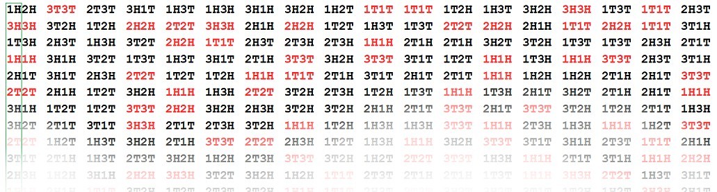
Words	Flap 1	Flap 2	Flap 3
Flap 1	100% are the same (`1T1T` or `1H1H`)	55% are the same (`1T2T` or `1H2H`)	61% are the same (`1T3T` or `1H3H`)
Flap 2	54% are the same (`2T1T` or `2H1H`)	100% are the same (`2T2T` or `2H2H`)	45% are the same (`2T3T` or `2H3H`)
Flap 3	55% are the same (`3T1T` or `3H1H`)	49% are the same (`3T2T` or `3H2H`)	100% are the same (`3T3T` or `3H3H`)

TABLE 3: Statistical properties of 432 word-pairs obtained with a classical experiment. Green boxes: probability
of getting the same words for the 293 word-pairs with different flap-numbers.

The analysis is therefore compatible with the predicted probability of 50%.

A quantum experiment

5) Quantum experiment

The experimental setup is described here for reference only. More details can be found in original papers such as in [3] but are very specialized. It is best to think of this description in terms of black boxes and compare it with the classical scenario described above. As with the classical scenario, the quantum experiment has two receivers (called A and B), a choice between three possible measurements (called 1, 2, or 3) and only two possible outcomes (called H or T).

A real quantum experiment can be made using a system with a single Source and two Detectors. The Source emits a pair of simultaneous light-pulses in opposite directions: one light-pulse toward Detector A and the other toward Detector B (see Figure A).

The detectors measure the polarization of the light-pulses using an analyzer and two photodetectors. When a photodetector detects a light-pulse, it amplifies the signal to produce an electrical output large enough to be easily measured. The analyzer redirects the light-pulses according to their polarization: If a light-pulse goes through the analyzer, the photodetector labeled "heads" generates an output; if a light-pulse is reflected by the analyzer, the photodetector labeled "tails" generates an output. It is possible to produce light-pulses which will only trigger one photodetector at a time. Either "heads" or "tails" will produce an output at "H" or "T" respectively, never both at the same time. Hence the name "photon" is used because the indivisible quantized light-pulse can't be split: it will either go straight into photodetector "heads" or be reflected into photodetector "tails".

FIGURE A: Simplified schematics of an experimental setup. Two Detectors measure the polarization of the received light.
The Source produces simultaneous photon-pairs.

After the photon-pair is emitted, the Detectors are rotated individually about the axis of the light beam. The entire assembly analyzer-photodetectors is rotated. The Detectors are set randomly to any of three positions:
Setting 1: aligned with the vertical at 0°,
Setting 2: rotated by 60° with respect to the vertical, or,
Setting 3: rotated by 120° with respect to the vertical.
Figure B shows an example with Detector A rotated by 60° and Detector B aligned with the vertical at 0°.

FIGURE B: Configuration with Detector A at Setting 2 and Detector B at Setting 1

6) Results and statistical analysis

When photon-pairs are detected, the settings of the Detectors are recorded with the observed output-pairs. A list of output-pairs is produced which uses the same notation used for the classical experiment described above. For example, 2T1H means that Dectector A was set to 2 and measured a photon on "tails", and Detector B was set to 1 and measured a photon on "heads".

Such a setup which uses the above concepts has been built Ref. [3].
The analysis of output-pairs gives the following results:

A) The probability for producing an output "heads" is 50% and the probability of obtaining "tails" is 50%.

B) The probability of the same outputs for an output-pair is near 100% with the same detector setting.

This analysis reveals that the quantum experiment produces probabilities compatible with the classical experiment for individual detector probabilities and for output-pairs with the same detector setting.

7) Model and comparison with experimental results

At this point, we have the same situation as with the classical experiment described above. The setting of the Detector corresponds to the flap-number. The outcomes "heads" or "tails" have the same statistical properties as those described in 2A and 2B for the classical experiment. We can therefore follow the same logic we followed in (3) to find the same model.
In this case, the model as described in (4) makes the same prediction for the quantum experiment:

When we chose a different setting for the Detectors, the probability of obtaining the same outputs in an output-pair must be 50%.

Comparison with experiment:
When the output-pairs from the quantum experiment Ref. [3] are analyzed, the following results are obtained which can be summarized in the following table:

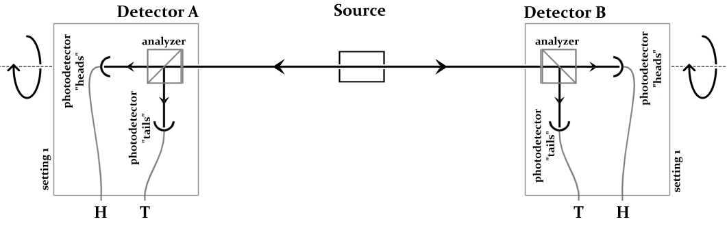
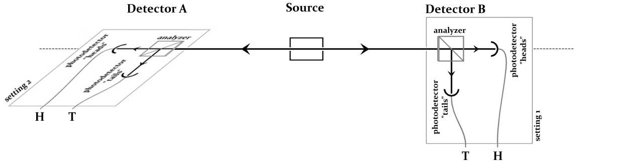
Outputs	Setting 1	Setting 2	Setting 3
Setting 1	>99% are the same	~25% are the same	~25% are the same
Setting 2	~25% are the same	>99% are the same	~25% are the same
Setting 3	~25% are the same	~25 % are the same	>99% are the same

TABLE 4: Statistical properties of measured occurrence of output-pairs. The results
obtained with the quantum experiment for different settings are not
compatible with the 50% predicted by the classical theory.

When the Detectors have different settings, the probability of getting the same outputs in an output-pair is near 25%. This is incompatible with the prediction of a probability of 50%. (Another experiment Ref. [4] uses 143 km between the emitter and receiver. It also shows incompatibility with the classical prediction, although the long distance introduces noise and reduces the probabilities to 80% for the same setting and 28% for different settings.)

It is as if one Detector knows that the other one does not have the same setting and, by some spooky action at a distance, is able to change the statistics of the measurements. This is, of course, impossible because the detector settings are chosen randomly a few microseconds before detection, a time too short to propagate any signal back to the other detector even at the speed of light.

Entanglement

Experimental results show that the classical model incorrectly predicts the statistical properties of quantum experiments. This implies that the assumptions that were used are incorrect: locality or reality are incompatible with quantum physics. This is what Bell showed formally in his 1964 paper.

Entanglement describes the statistical property resulting from only one element of reality for two separated signals and detectors at the same time, independent of the distance between the detectors. The signals reaching the detectors and the position of the detectors behave as a whole, even if the setting of one detector can be changed randomly just before a measurement made by the other detector. This has been verified experimentally.

Entanglement, as described by quantum mechanics, is a solution which predicts experimental results. However, it rejects "reality" (Einstein would not reject elements of reality!) and "locality" (Einstein called this spooky action at a distance!) This tells us that the behaviour of the quantum world is far from our common experience.

References

[1] David Mermin, "Is the moon there when nobody looks", Physics Today, pp. 38-47, April 1985.
[2] John Bell, "On the Einstein Podolsky Rosen Paradox," Physics. 1 (3), 195–200 (1964).
[3] Alain Aspect et al., "Experimental Test of Bell's Inequalities Using Time-Varying Analyzers", Physical Review Letters 45, no. 25, p. 1804, 20 Dec 1982.
[4] Xiao-song Ma et al., "Quantum teleportation over 143 kilometres using active feed-forward," Nature 489, 269–73 (2012), also https://arxiv.org/abs/1205.3909.